Cluster Sizing Case Study - Mirrored Queues Part 1
In a first post in this sizing series we covered the workload, cluster and storage volume configurations on AWS ec2. In this post we’ll run a sizing analysis with mirrored queues.
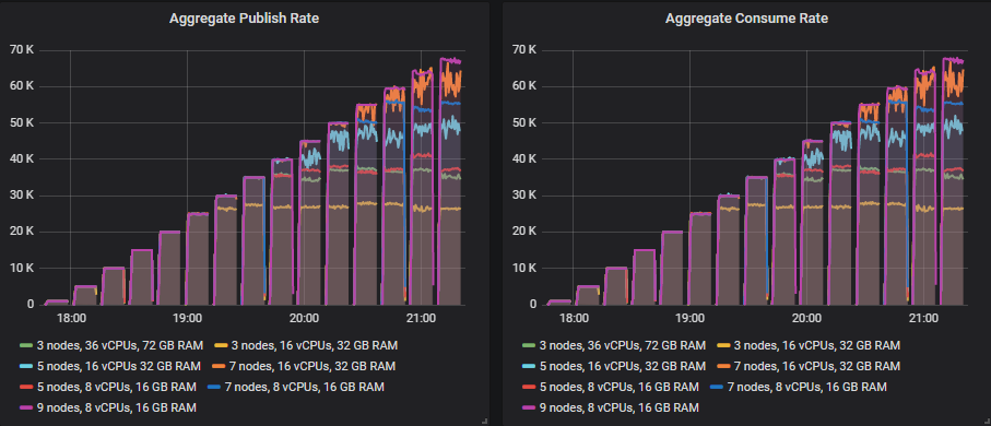
The first phase of our sizing analysis will be assessing what intensities each of our clusters and storage volumes can handle easily and which are too much.
All tests use the following policy:
- ha-mode: exactly
- ha-params: 2
- ha-sync-mode: manual
Ideal Conditions - Growing Intensity Tests
In a previous post we discussed options for running benchmarks. You can run this workload, at these intensities with the following command:
bin/runjava com.rabbitmq.perf.PerfTest \
-H amqp://guest:guest@10.0.0.1:5672/%2f,amqp://guest:guest@10.0.0.2:5672/%2f,amqp://guest:guest@10.0.0.3:5672/%2f \
-z 1800 \
-f persistent \
-q 1000 \
-c 1000 \
-ct -1 \
--rate 50 \
--size 1024 \
--queue-pattern 'perf-test-%d' \
--queue-pattern-from 1 \
--queue-pattern-to 100 \
--producers 200 \
--consumers 200 \
--consumer-latency 10000 \
--producer-random-start-delay 30
Just change the --rate argument to the rate you need for each test and remember that it is the rate per publisher rather than the total combined rate. Because the consumer processing time (consumer latency) is set to 10ms, we also need to increase the number of consumers for the higher publish rates.
Before running PerfTest you will need to create a policy to turn the created queues into mirrored queues with one master and the number of mirrors you wish to test with.
io1 - High Performance SSD
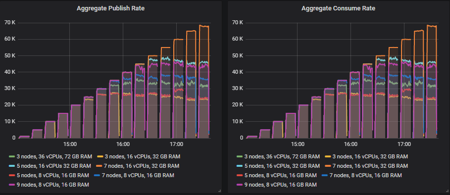
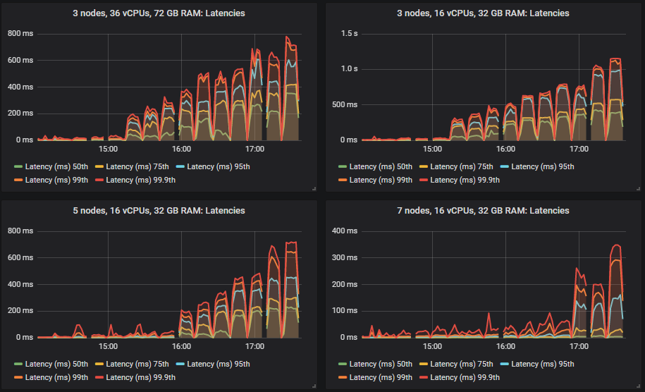
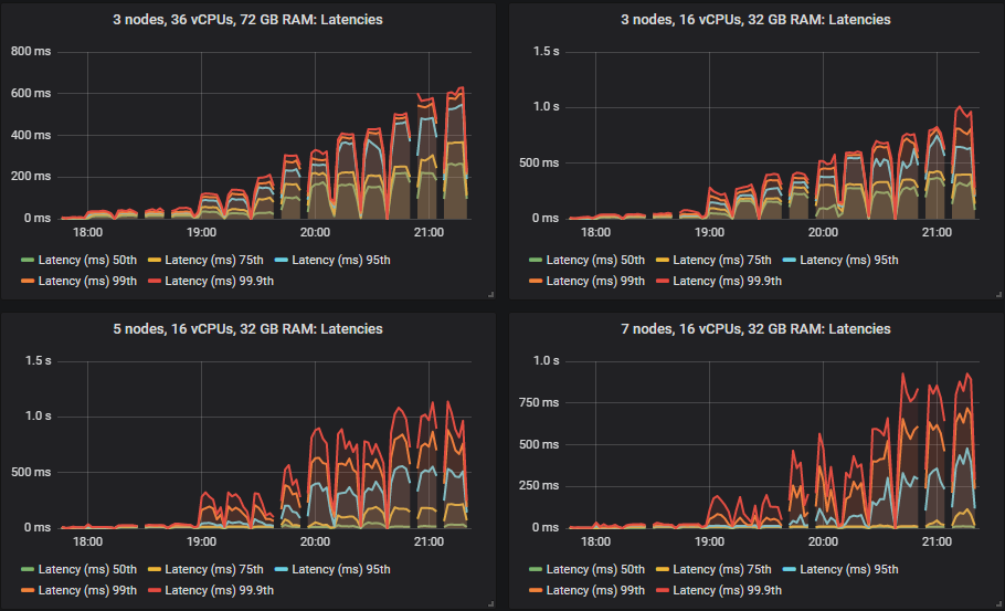
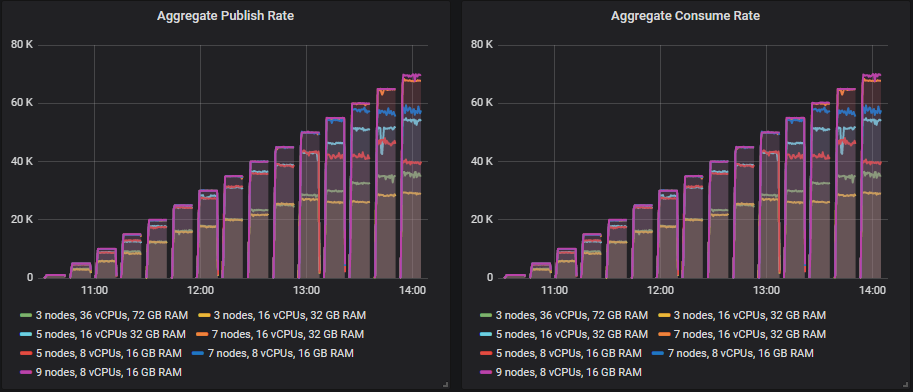
Different clusters managed to reach different intensities but all tests except for one remained under the 1 second for 99th percentile end-to-end latency requirement.
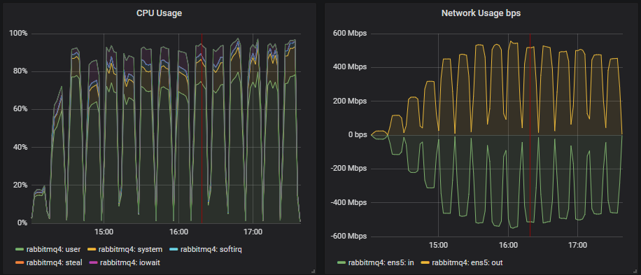
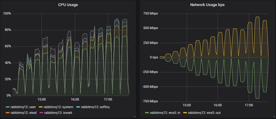
The limiting factor in most tests was CPU so no surprise that the configuration with most CPUs did best. What was interesting is that the 3 node, 36 vCPU cluster (3x36) that had the second highest total vCPU count was way down, below the 7x8 vCPU cluster. In fact, CPU didn’t go above 50% on the 3x36 cluster, it seems that Erlang was not able to efficiently make use of all those 36 vCPUs per broker (more on that later).
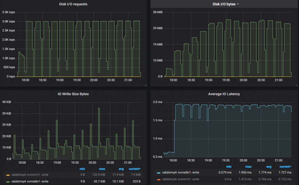
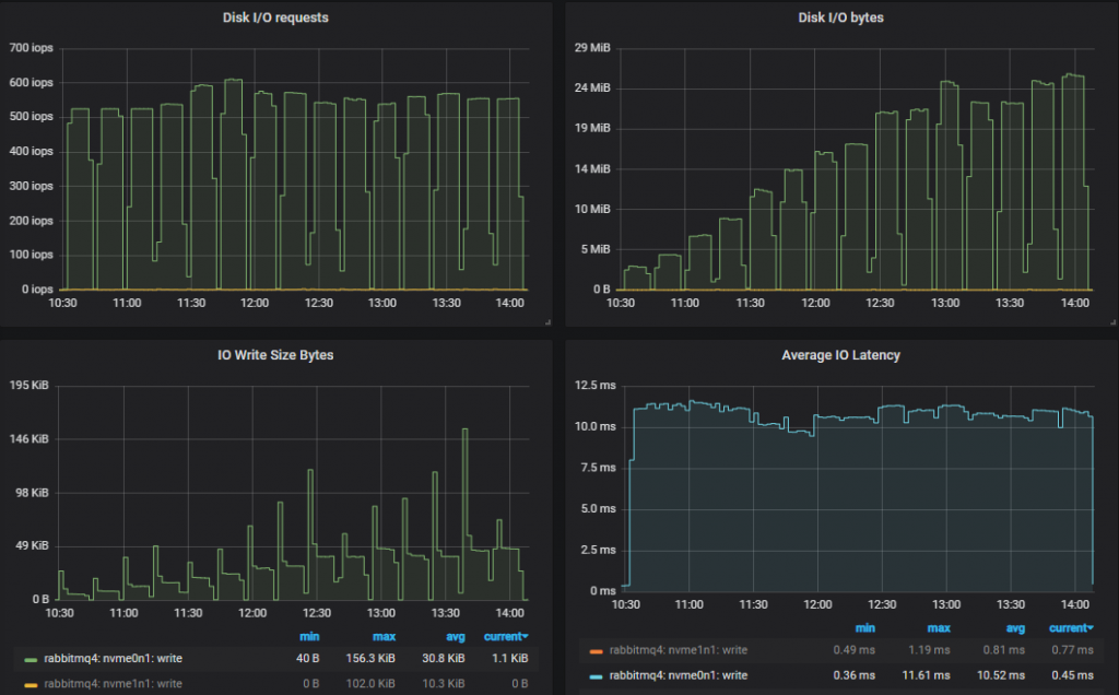
Disk throughput did not get close to capacity, but IOPS did reach 8000-9000 in all configurations with roughly 5-7kb write sizes. Network bandwidth remained lower than 1gbit, which was within the limit of all VMs.
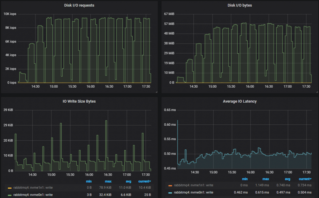
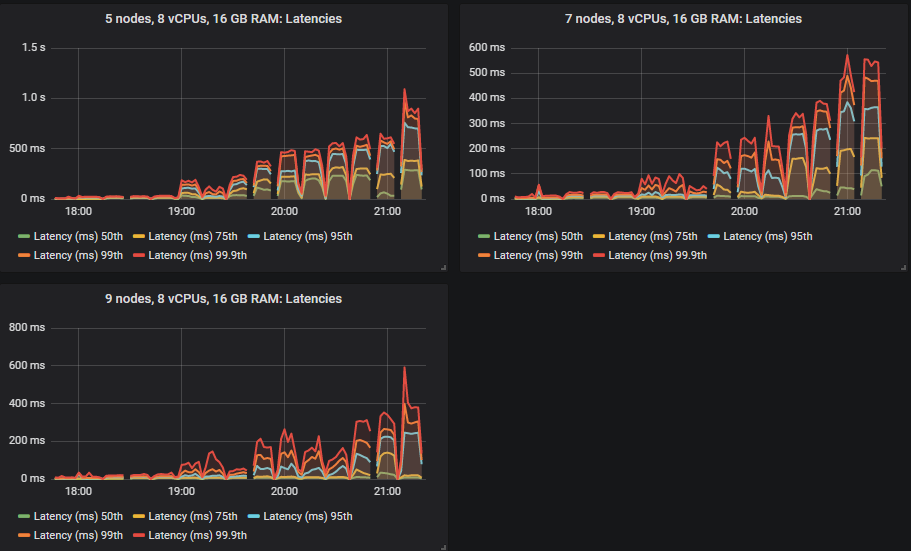
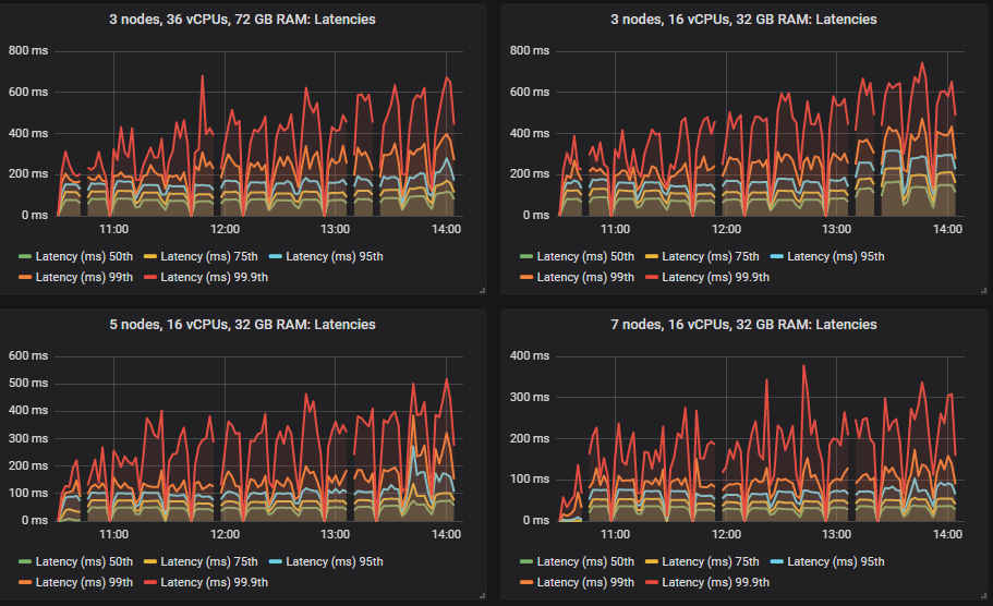
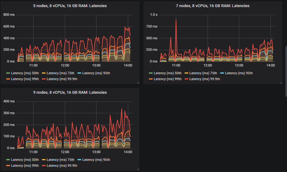
Bottom throughput cluster (3x16):
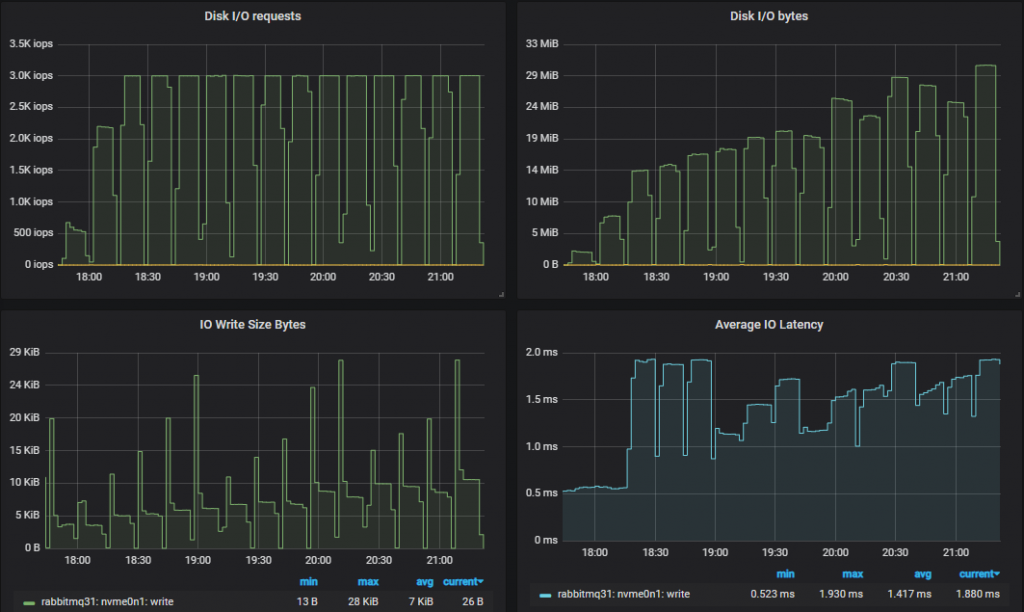
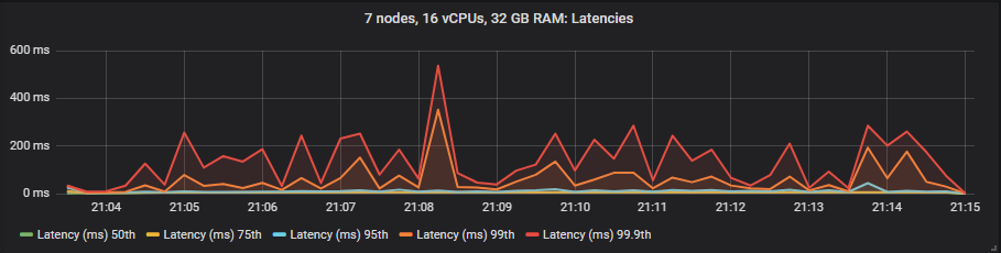
Top throughput cluster (7x16)
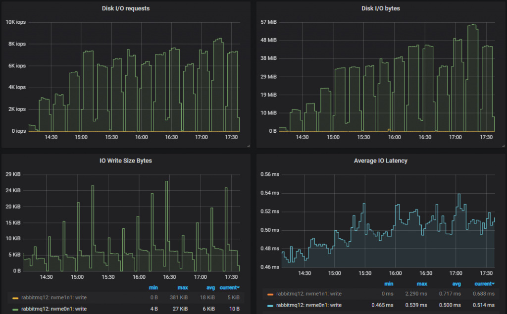
Insight: The lower performing 3x16 cluster had a slightly higher disk write throughput than the top performing 7x16 cluster. This is because a message is not persisted to disk if it has already been consumed by the time an fsync is performed. So when consumers keep up, disk writes are lower. If we look at the 25k msg/s test which is the highest both can handle, we see that the 3x16 cluster has a 95th percentile latency of around 250ms and the 7x16 around 4ms. Fsyncs occur every 200ms roughly. So the higher performing cluster performs less writes.
Leaderboard in matched target throughput
The highest throughput each cluster size managed, where it delivered exactly the target rate.
- Cluster: 7 nodes, 16 vCPUs (c5.4xlarge). Rate: 65k msg/s
- Cluster: 5 nodes, 16 vCPUs (c5.4xlarge). Rate: 45k msg/s
- Cluster: 9 nodes, 8 vCPUs ( c5.2xlarge). Rate: 45k msg/s
- Cluster: 7 nodes, 8 vCPUs (c5.2xlarge). Rate: 40k msg/s
- Cluster: 3 nodes, 36 vCPUs (c5.9xlarge). Rate: 30k msg/s
- Cluster: 5 nodes, 8 vCPUs (c5.2xlarge). Rate: 20k msg/s
- Cluster: 3 nodes, 16 vCPUs (c5.4xlarge). Rate: 20k msg/s
We see the middle ground of scaling up and out gave us the best throughput but scaling out did pretty well too. Scaling up was not so good.
Leaderboard in cost per 1000 mgs/s per month, at top throughput.
- Cluster: 5 nodes, 16 vCPUs. Cost: $134 (45k msg/s)
- Cluster: 7 nodes, 16 vCPUs. Cost: $140 (65k msg/s)
- Cluster: 7 nodes, 8 vCPUs. Cost: $170 (40k msg/s)
- Cluster: 3 nodes, 16 vCPUs. Cost: $182 (20k msg/s)
- Cluster: 3 nodes, 36 vCPUs. Cost: $182 (30k msg/s)
- Cluster: 9 nodes, 8 vCPUs. Cost: $194 (45k msg/s)
- Cluster: 5 nodes, 8 vCPUs. Cost: $242 (20k msg/s)
Leaderboard in cost per 1000 msg/s per month at a target of 30k msg/s.
- Cluster: 3 nodes, 36 vCPUs. Cost: $183
- Cluster: 5 nodes, 16 vCPUs. Cost: $202
- Cluster: 7 nodes, 8 vCPUs. Cost: $226
- Cluster: 9 nodes, 8 vCPUs. Cost: $291
- Cluster: 7 nodes, 16 vCPUs. Cost: $307
While scaling out with smaller VMs had decent throughput, it was undermined by the fact that our disks were the most expensive item. Because the disks were expensive, the most cost effective cluster was the one with the least instances, however, this 3x36 cluster only just managed the peak in this ideal conditions test, it is unlikely to hold up under the more difficult tests. So if we ignore the 3x36 cluster, the most cost effective was the middle ground of scaling up and out.
Do we really need those costly io1 SSDs? We’re not needing them for IO throughput, but those 10000 IOPS are almost fully utilised. Will the 3000 IOP gp2 handle the higher intensities?
gp2 - General Purpose SSD
Again, different clusters managed different throughputs, but all came in within the end-to-end latency requirements.
We have a new winner with the gp2 volume: the 9x8 cluster followed by the 7x8 cluster. The 7x16 and 5x16 showed some choppy throughput once they had reached and then past their top capacity. The bottom two were the same: the 3x36 and 3x16 clusters.
So how did RabbitMQ handle the lower IOPs volumes?
Bottom Throughput Cluster (3x16)
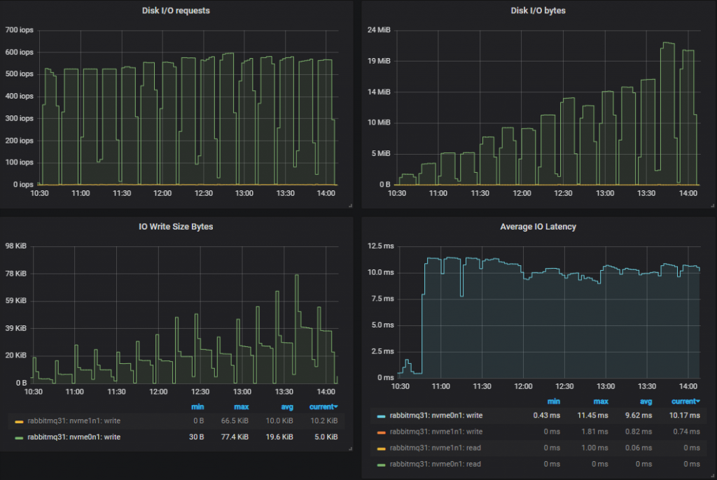
We hit the 3000 IOPs limit from the 5000 msg/s rate and upward. As the tests go on, in order to cope with the larger disk throughput, the IO size increases. So it looks like we don’t need all those IOPs after all.
Top Throughput Cluster (9x8)
Exactly the same story for the highest performing cluster - RabbitMQ adjusted to the lower available IOPs.
Leaderboard in matched target throughput
- Cluster: 9 nodes, 8 vCPUs (c5.2xlarge). Rate: 65k msg/s
- Cluster: 7 nodes, 8 vCPUs (c5.2xlarge). Rate: 50k msg/s
- Cluster: 7 nodes, 16 vCPUs (c5.4xlarge). Rate: 50k msg/s
- Cluster: 5 nodes, 16 vCPUs (c5.4xlarge). Rate: 40k msg/s
- Cluster: 3 nodes, 36 vCPUs (c5.9xlarge). Rate: 35k msg/s
- Cluster: 5 nodes, 8 vCPUs (c5.2xlarge). Rate: 35k msg/s
- Cluster: 3 nodes, 16 vCPUs (c5.4xlarge). Rate: 25k msg/s
This time, scaling out was clearly the most effective. Scaling up was not so good.
Leaderboard in cost per 1000 messages per month, at top throughput.
- Cluster: 9 nodes, 8 vCPUs. Cost: $48 (65k msg/s)
- Cluster: 7 nodes, 8 vCPUs. Cost: $48 (50k msg/s)
- Cluster: 5 nodes, 8 vCPUs. Cost: $49 (35k msg/s)
- Cluster: 3 nodes, 16 vCPUs. Cost: $71 (25k msg/s)
- Cluster: 5 nodes, 16 vCPUs. Cost: $74 (40k msg/s)
- Cluster: 7 nodes, 16 vCPUs. Cost: $96 (50k msg/s)
- Cluster: 3 nodes, 36 vCPUs. Cost: $103 (35k msg/s)
In terms of cost per top throughput the order was: core count desc, node count desc.
Leaderboard in cost per 1000 messages per month at a target of 30k msg/s.
- Cluster: 5 nodes, 8 vCPUs. Cost: $58
- Cluster: 7 nodes, 8 vCPUs. Cost: $81
- Cluster: 5 nodes, 16 vCPUs. Cost: $98
- Cluster: 9 nodes, 8 vCPUs. Cost: $104
- Cluster: 3 nodes, 36 vCPUs. Cost: $120
- Cluster: 7 nodes, 16 vCPUs. Cost: $161
At our target rate of 30k msg/s, the 5x8 was the best. The conclusion is that scaling out smaller VMs gave both better performance but also best cost effectiveness. The reason was that the gp2 volumes are relatively cheap and we don’t get penalised for scaling out like we did with the expensive io1 volumes.
st1 - HDD
So far we’ve seen RabbitMQ make use of the available IOPs it has available by adjusting to lower IOPs as needed. HDDs are built for large and sequential workloads with low IOPs so will RabbitMQ be able to adjust its disk operations yet again to make even fewer, but larger disk operations? Let’s see.
Looking at the throughput, HDDs did the best of all in terms of top throughput, actually achieving the 70k msg/s highest intensity. The end-to-end latency had a different pattern. With the SSDs the latencies started out very small and then grew as the intensity grew. But the HDDs started out with a much higher latency and it grew at a much lower rate.
Let’s see how RabbitMQ used the available IOPs.
Bottom Throughput Cluster (3x16)
We’re down now to 500-600 IOPS with an average write size approaching 50kb (ignoring the initial peaks). Far fewer, but much larger IO operations. IO latency is much higher. We’ve gone from 0.5ms (io1), 2ms (gp2) to 10ms (st1) which is likely a combination of the IO size and ability of the storage drive to do random IO fast. Further down, we’ll compare end-to-end latency for the three disk types.
Top Throughput Cluster (9x8)
Leaderboard in throughput
Only three sizes were able to meet their targets, the rest were always short, even as their throughput climbed in each test. We might have been able to increase throughput with different publisher confirm in-flight limits, a higher limit might have benefited the higher latency HDDs.
The winners that were able to hit their target were:
- Cluster: 9 nodes, 8 vCPUs (c5.2xlarge). Rate: 70k msg/s
- Cluster: 7 nodes, 16 vCPUs (c5.4xlarge). Rate: 65k msg/s
- Cluster: 7 nodes, 8 vCPUs (c5.2xlarge). Rate: 55k msg/s
The rest fell short of their targets in each test, but still showed higher throughput as the tests progressed:
- Cluster: 5 nodes, 16 vCPUs (c5.4xlarge). Rate: 55k msg/s
- Cluster: 5 nodes, 8 vCPUs (c5.2xlarge). Rate: 43k msg/s
- Cluster: 3 nodes, 36 vCPUs (c5.9xlarge). Rate: 35k msg/s
- Cluster: 3 nodes, 16 vCPUs (c5.4xlarge). Rate: 29k msg/s
With HDDs, it was all about scaling out, not up.
Leaderboard in cost per 1000 messages per month, at their top rate.
- Cluster: 5 nodes, 8 vCPUs. Cost: $65 (43k msg/s)
- Cluster: 7 nodes, 8 vCPUs. Cost: $71 (55k msg/s)
- Cluster: 9 nodes, 8 vCPUs. Cost: $72 (70k msg/s)
- Cluster: 5 nodes, 16 vCPUs. Cost: $73 (55k msg/s)
- Cluster: 3 nodes, 16 vCPUs. Cost: $83 (29k msg/s)
- Cluster: 7 nodes, 16 vCPUs. Cost: $97 (65k msg/s)
- Cluster: 3 nodes, 36 vCPUs. Cost: $121 (35k msg/s)
Leaderboard in cost per 1000 messages per month at a target of 30k msg/s.
- Cluster: 5 nodes, 8 vCPUs. Cost: $93
- Cluster: 7 nodes, 8 vCPUs. Cost: $131
- Cluster: 5 nodes, 16 vCPUs. Cost: $134
- Cluster: 3 nodes, 36 vCPUs. Cost: $142
- Cluster: 9 nodes, 8 vCPUs. Cost: $168
- Cluster: 7 nodes, 16 vCPUs. Cost: $211
In terms of their top throughput, its clear that smaller VMs were most cost effective. But when considering the target of 30k msg/s, the middle ground of scaling out/up showed the best results. There is some conflict again between scaling out which is best for performance and cost (the st1 volumes are a little costly). So the middle ground wins.
End-to-end Latency and the Three Volume Types
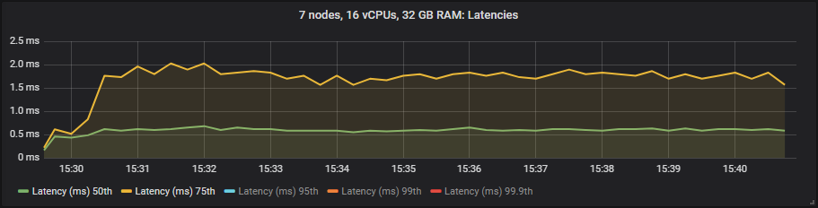
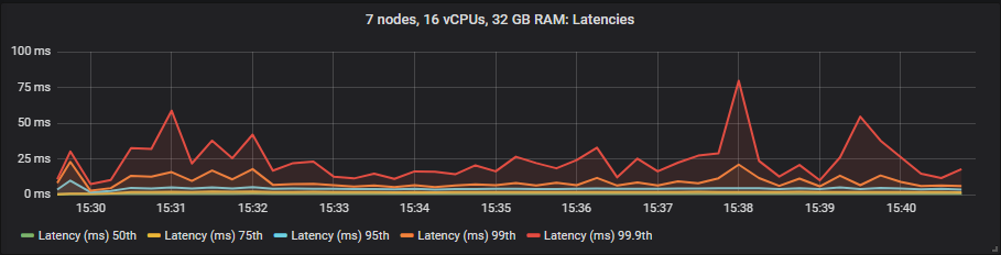
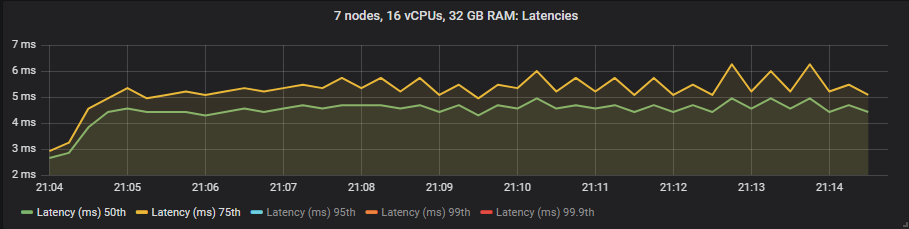
In these tests we treat end-to-end latency as the time between a message being published and consumed. If we look at the 30k msg/s target rate and the 7x16 cluster type we see:
io1
gp2
st1
We see that io1 delivers the best latencies up to 95th percentile, after that it matched more or less gp2. The st1 HDD showed much higher in latencies but still within our target of 1 second.
CPU Utilisation and 36 vCPU VMs
In the 8 and 16 vCPU (CPU thread) instances, CPU seems to be the bottleneck. Once CPU reached above 90% we stopped seeing any more increases in throughput. However, the 36 vCPU instances tended to always look like this:
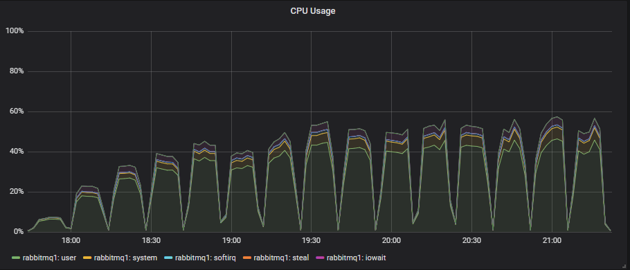
CPU utilisation and Erlang is not always straightforward. Erlang schedulers will do busy-waiting when they deem that it is more effective to do so. This means that rather than sleep, a scheduler sits in a busy loop, utilising CPU while it waits for new work to do. This can make it appear that the Erlang application is doing lots of work, using the CPU, but actually it is just waiting for work.
36 vCPUs is just a waste in this particular case. We’ve seen that they are more expensive and deliver inferior results compared to scaled out smaller VMs.
Increasing Intensity Benchmarks - Conclusion
So far the conclusions are:
- The expensive io1 is only worth it if we really care about end-to-end latency.
- The inexpensive gp2 offers the best combination of performance and cost and is the best option for most workloads. Just remember that we used a 1TB size that does not have burst IOPs and there is a 250 MiBs limit (which we never hit).
- With cheap storage volumes, scaling out the smaller 8 vCPU VMs was the most cost effective and best in terms of performance.
- With expensive volumes, going with the middle ground of scaling out and up was most cost effective.
- CPU utilisation seemed to be the limiting factor on the 16 and 8 vCPUs. The large 36 vCPU instances didn’t go past 60% utilisation, but also didn’t hit disk or network limits. Erlang just couldn’t efficiently use that many cores.
Top 5 Configurations for cost per 1000 msg/s per month for the 30k msg/s throughput:
- Cluster: 5 nodes, 8 vCPUs, gp2 SDD. Cost: $58
- Cluster: 7 nodes, 8 vCPUs, gp2 SDD. Cost: $81
- Cluster: 5 nodes, 8 vCPUs, st1 HDD. Cost: $93
- Cluster: 5 nodes, 16 vCPUs, gp2 SDD. Cost: $98
- Cluster: 9 nodes, 8 vCPUs, gp2 SDD. Cost: $104
We've only tested under ideal conditions...
We've gathered a lot of data from 21 different cluster configurations at 15 different workload intensities. We think that so far we should go with a medium to large cluster of small VMs on the inexpensive gp2 volumes. But this was testing the happy scenario where queues are empty or close to empty where RabbitMQ operates at its peak performance. Next we'll run more tests that ensure that despite brokers being lost and queue backlogs occurring that our chosen cluster size continues to deliver the performance that we need. Next we test resiliency.